Processing the angles and angular momentum in sheared granular material simulations ↩

aliases: []
shorthands: {}
created: 2022-07-11 14:33:24
modified: 2022-07-11 15:27:17

Let's look at an example. Similarly to in the other method regarding the angles of grains, we load the list of files first and determine the shape of the ellipsoidal particles:

import os

foldername = "0.0854988_0.0854988_0.341995"
files = os.listdir(f"../outfiles/{foldername}/")
[a, b, c] = list(map(float, foldername.split('_')))
is_z_longest = np.argmax([a, b, c]) == 2

We also again need a way of filtering out the shear zone. We use the simplest method for this:

from scipy import optimize

def vel_estimator_func(coord, transition_rate, y_displacement, x_lin, x_quad, z_lin, z_quad):
    x = coord[0]
    y = coord[1]
    z = coord[2]
    return np.tanh(y_displacement + (y + x*x_lin + x*x*x_quad + z*z_lin + z*z*z_quad)*transition_rate)


def vel_estimator_func_derivative_y(coord, transition_rate, y_displacement, x_lin, x_quad, z_lin, z_quad):
    return transition_rate * (1 - vel_estimator_func(coord, transition_rate, y_displacement, x_lin, x_quad, z_lin, z_quad)**2)


def filter_shear_zone(coords, vs):
    fitParams, fitCovariances = optimize.curve_fit(
        vel_estimator_func, [coords[:, 0], coords[:, 1], coords[:, 2]], vs[:, 0])

    gradient_from_fit = - \
        vel_estimator_func_derivative_y(
            [coords[:, 0], coords[:, 1], coords[:, 2]], *fitParams)

    zone_filter = gradient_from_fit < -1.3

    return zone_filter, fitParams

Where filter_shear_zone is modified to return the final parameters of the fitting for later use.

Then we can iterate through all the files and aggregate the data. In each iteration, we have to get the angles, like in Determining angle distribution in shear zones in granular material simulations and the -components of the angular momentum as well.

import numpy as np
import vtkmodules.all as vtk
from vtkmodules.util.numpy_support import vtk_to_numpy
import re

all_shear_angles = np.array([], dtype=np.float64)
all_shear_omegazs = np.array([], dtype=np.float64)
all_shear_derivatives_y = np.array([], dtype=np.float64)

for file in files:
    # Filter filenames and load them
    res = re.search(r"dump\d+\.superq\.vtk", file)
    if not res:
        continue
    filename = file

    # Load file with vtk reader
    reader = vtk.vtkPolyDataReader()
    reader.SetFileName(f"../outfiles/{foldername}/{filename}")
    reader.Update()
    output = reader.GetOutput()

    # Store the needed data from the output file
    coords = vtk_to_numpy(output.GetPoints().GetData())
    vs = vtk_to_numpy(output.GetPointData().GetArray(3))
    orientations = vtk_to_numpy(output.GetPointData().GetArray(8))
    angular_momenta = vtk_to_numpy(output.GetPointData().GetArray(4))
    omegaz = angular_momenta[:, 2]

    # Filter the shear zone with the previously shown function
    zone_filter, fit_params = filter_shear_zone(coords, vs)
    filtered_orientations = orientations[zone_filter]
    filtered_vectors = filtered_orientations[:, [2, 5, 8]]
    # If the grains are flat, use the angle of the rotated vector
    if not is_z_longest:
        tmp_vals = np.copy(filtered_vectors[:, 0])
        filtered_vectors[:, 0] = -filtered_vectors[:, 1]
        filtered_vectors[:, 1] = tmp_vals
    # Flip vector if orientation in inverted
    filtered_vectors[filtered_vectors[:, 0] < 0] *= -1
    filtered_angles = np.arctan2(
        filtered_vectors[:, 1], filtered_vectors[:, 0])
    # Applt filter to other quantities as well
    filtered_omegazs = omegaz[zone_filter]
    filtered_coords = coords[zone_filter]
    filtered_derivatives_y = vel_estimator_func_derivative_y(
        filtered_coords.T, *fit_params)

    # Append retieved quantities
    all_shear_angles = np.append(all_shear_angles, filtered_angles)
    all_shear_omegazs = np.append(all_shear_omegazs, filtered_omegazs)
    all_shear_derivatives_y = np.append(
        all_shear_derivatives_y, filtered_derivatives_y)

With this loop, we collected all relevant information in the arrays all_shear_angles, all_shear_omegazs and all_shear_derivatives_y.
The shear rate = -derivative/gradient of the velocity is needed since we have to normalize the angular velocity with the shear rate for it to be universal (see Jeffery rotation), so the relevant array will be all_shear_omegazs / all_shear_derivatives_y.

Now we can then take the 2D histogram of the relevant quantities:

import plotly.express as px

# Create 100 x 500 histogram with numpy
image, xedges, yedges = np.histogram2d(
    all_shear_angles*(180 / np.pi), all_shear_omegazs/all_shear_derivatives_y, [100, 500])
# Determine the middl of the bins
xmids = (xedges[:-1] + xedges[1:]) / 2
ymids = (yedges[:-1] + yedges[1:]) / 2

# We want to norm on a per-column basis, to see all the detail in the graph
norms = np.linalg.norm(image, axis=1)
image = image / norms[:, None]

# Plot with plotly
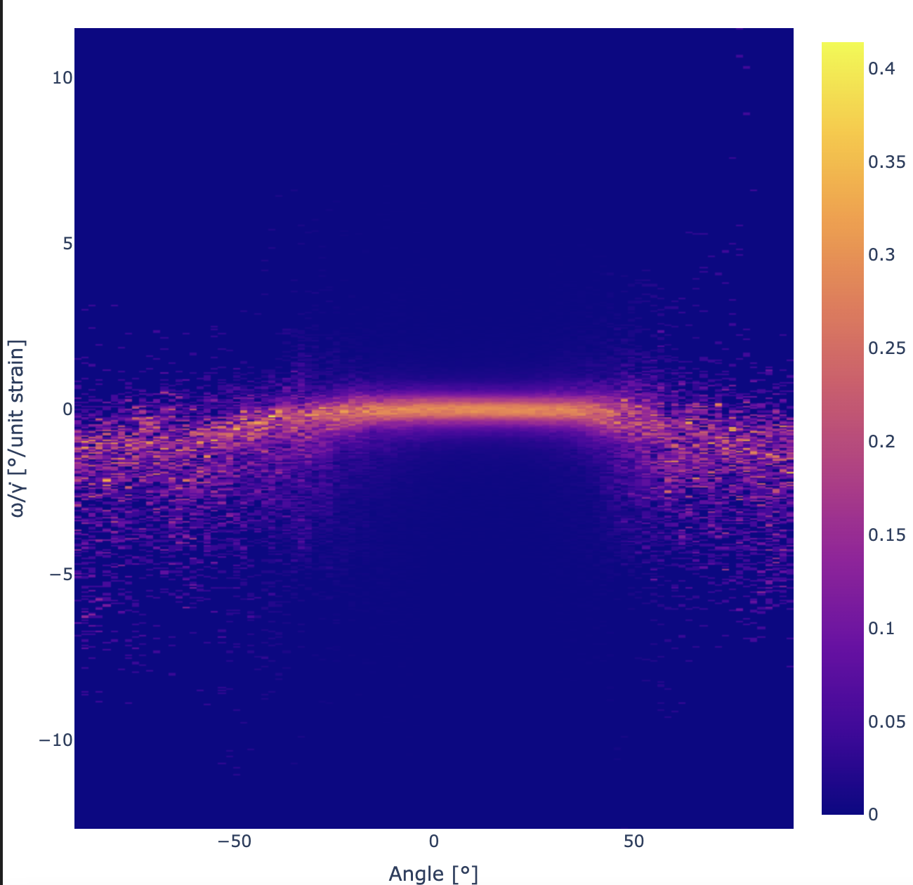
fig = px.imshow(image.T, x=xmids, y=ymids, aspect="square")
fig.update_layout(width=650, height=650, margin=dict(
    l=0, r=0, b=0, t=40), title="", scene_aspectmode='cube')
fig.update_yaxes(autorange=True)
fig.update_layout(xaxis_title="Angle [°]", yaxis_title="ω/γ̇[°/unit strain]")
fig.show()

Which results in the following graph:

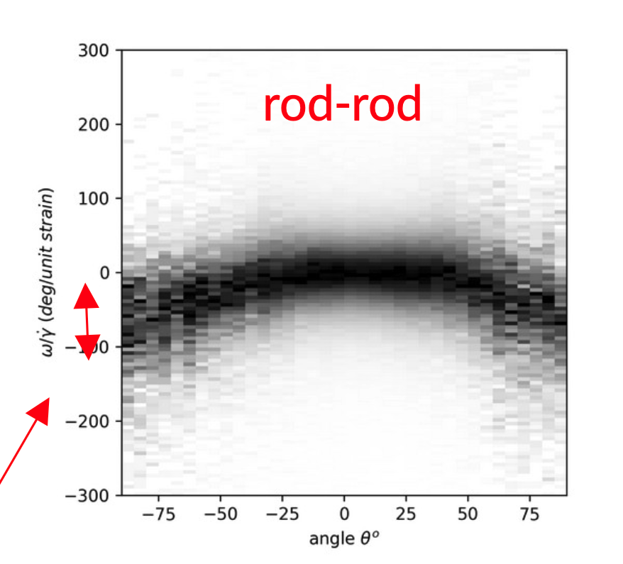
This graph is incredibly similar to the ones seen in real experiments, like this:

Per-column average and variance

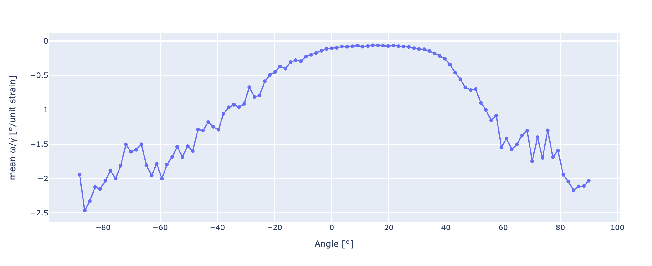
We can get a line graph from the following figure if we take its weighted average on a per-column basis (like calculating a center of mass in 1D). This can be done the following way:

krd = np.tile(ymids, (len(xmids), 1))
avgs = np.average(krd, axis=1, weights=image)
difference = np.subtract(krd, avgs[:, None])
# We can also calculate the variances and so the deviations
variances = np.average((difference)**2, axis=1, weights=image)
deviations = np.sqrt(variances)

fig = px.line(y=avgs, x=xedges[1:], markers=True)
fig.update_layout(xaxis_title="Angle [°]",
                  yaxis_title="mean ω/γ̇ [°/unit strain]")
fig.show()

Which results in:

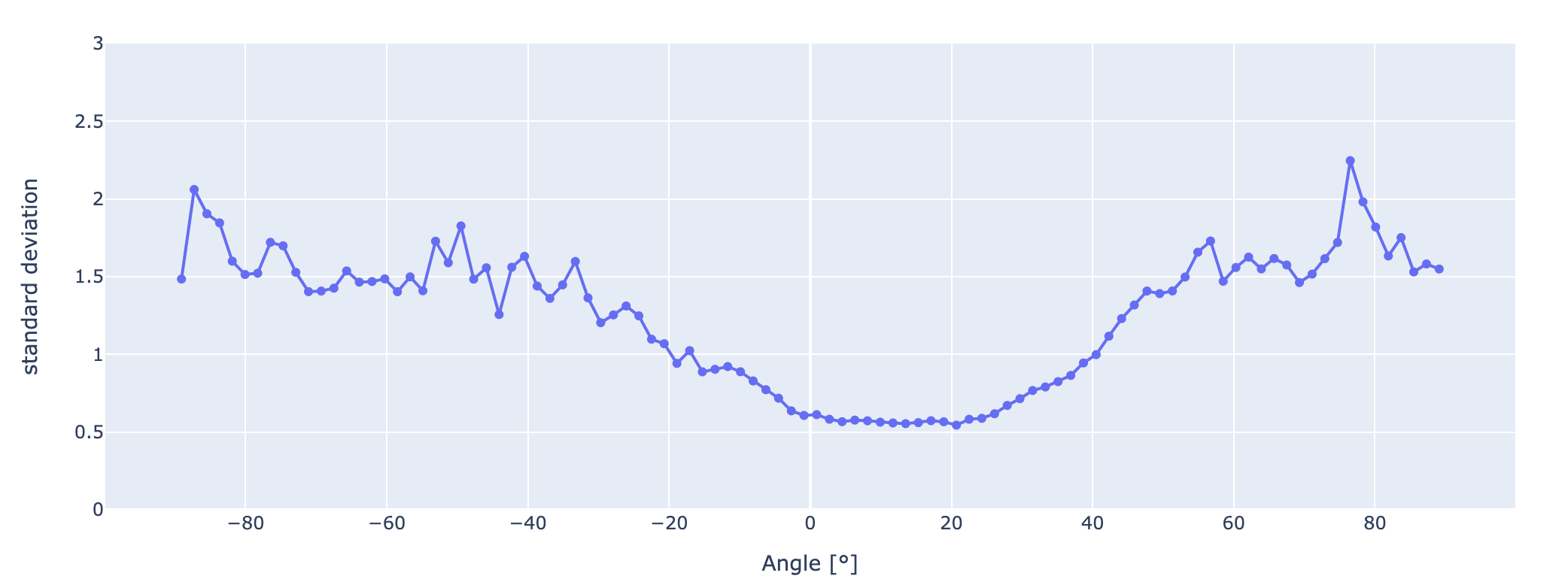
And now the variance and thus the deviation is easy to plot:

fig = px.line(y=deviations, x=xmids, markers=True)
fig.update_layout(yaxis_range=[0, 3])
fig.update_layout(xaxis_title="Angle [°]", yaxis_title="standard deviation")
fig.show()